日本語話者データ(米国)

英語版 English Version

🚧 工事中 🚧

なぜ

There are a number of factors unique to Japanese that create upward wage pressure for bilingual speakers.

需要側からは:

  1. 日本は米国に対する対外直接投資が最も多い国。1, 2
  2. GDP統計で日本は第4位(投資対象国), 購買力平価(PPP)調整では第5位3 4

供給側からは:

  1. 日本は(EF英語習熟度指数)で低い順位 5
  2. 日本語は他の言語より、英語との違いが多い。アラブ語、中国語、韓国語とともにもっとも習得が難しい言語と言われてます。6
  3. 他の国と比べると日本から移住する人数は少ない(均等割り) 7
  4. 米国内の地域による集積や不均衡 8

データ

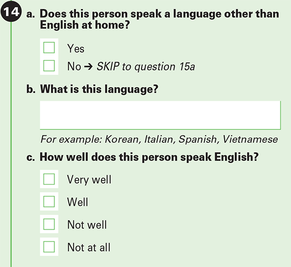
ACS(調査)の問題:

https://data.census.gov/からのデータ
  参考文献:
U.S. Census Bureau. “Language Spoken at Home by Ability to Speak English for the Population 5 Years and Over.” American Community Survey, ACS 5-Year Estimates Detailed Tables, Table B16001.

調査の全体: https://www.census.gov/programs-surveys/acs/about/forms-and-instructions.html

データに注意する問題点:

  • The errors are based on a 90% confidence interval.
  • ACS data is not a census and may suffer from non-sampling error.
  • Data is for all age groups when one might only be interested in those of working age (18-64) my best estimate puts it at ~60%.
  • The bilingual statistic is based on those who responded as speaking english “very well”, excluding those who selected as speaking “well” or below.
  • Individuals who know the language may interpret “speak language at home” more strictly and not respond with the language spoken. ie. A language learner w/o someone to speak w/ at home.
  • Speaking at home is used as a proxy to fluency, but such fluency may be considered insufficient by other standards. (尊敬語 or reading/writing skills come to mind)

Observations

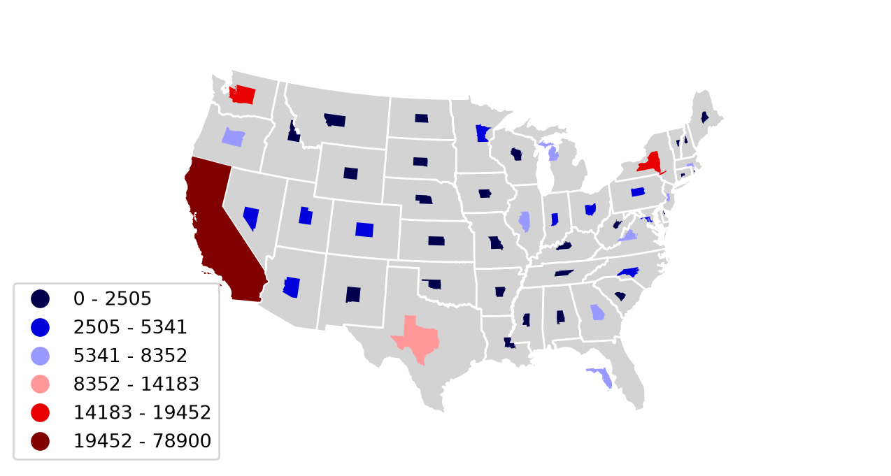
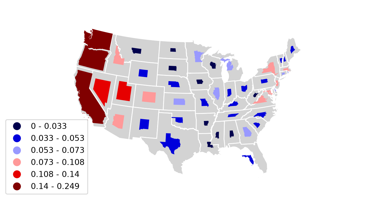
Hawaii has the highest proportion of Japanese, but due to size Hawaii actually has fewer bilingual speakers than the NYC metro area (20552 Bilingual speakers in Hawaii; 23268 Bilingual speakers in NY-NJ metro area).

Alaska, Utah, Nevada stood out as locations not traditionally associated with a Japanese diaspora, but had relatively high populations of Japanese speakers.

Florida and Texas have a low proportion of Japanese speakers, but make up for it by sheer size.

表・見える化

Code
import pandas as pd
import geopandas as gpd
import numpy as np
import folium
import itables
import geoplot
import mapclassify as mc
import geoplot.crs as gcrs
import matplotlib

jpmap = gpd.read_file("../../census/jpmap.gpkg")
itables.options.css = """
.dt-column-header {
  font-size: small;
}
"""
jtable = jpmap.loc[:,["ST","state","population","epopulation","eng","eeng","jpn","ejpn","bilingual","ebilingual",
                            "jpnloweng","ejpnloweng","pctjpn","pctbilingual","bilingualratio"]]
jtable.columns = ["州(略)","州","人工","人工(誤差)","英語人","英語人(誤差)","日本語人","日本語人(誤差)","日英バイリン","日英バイリン(誤差)", 
                            "英下手","英下手(誤差)","日本語比率","バイリン比率","バイリン割り"]
itables.show(pd.DataFrame(jtable), 
                            maxBytes=200000, style="width:100%", 
                            buttons=["pageLength", {"extend": "colvisGroup","text": "誤差を隠す","hide": [0,3,5,7,9,11]},
                                                    {"extend": "colvisGroup","text": "全体","show": "*"}],
                            columnDefs=[{"className":"dt-left", "targets":[0,1]}, 
                                        {"targets":[0,3,5,7,9,11], "visible":False}],
                            columnControl=["order"],
                            ordering={"indicators": False, "handler": False})
ⓘ州(略) 州 人工 人工(誤差) 英語人 英語人(誤差) 日本語人 日本語人(誤差) 日英バイリン 日英バイリン(誤差) 英下手 英下手(誤差) 日本語比率 バイリン比率 バイリン割り
ALalabama4793030601450321853592528541122841413003270.0527430.02562148.575949
AKalaska6890701695851622727149439010332814612540.2168140.14991269.143240
AZarizona69813202855184054115447952907511970628335110.1139040.07332464.373742
ARarkansas2869111548263045144419352664951954402180.0325880.01725352.941176
CAcalifornia37121454487206426385445013341945947890031905451922220.3594120.21254659.137004
COcolorado5549558577465028392235893658449456313992660.1061890.08097976.259969
CTconnecticut34428179026383666723328164023225049593290.0953000.06744570.771106
DEdelaware9665804682033634328052726032292021020.0832830.06238574.906832
DCdistrict of columbia64084166518478320410542856922443621450.1644710.10798365.654649
FLflorida212897287071476945825976122221183815399340696470.0574080.03829566.707577
(41 more rows not shown)
Code
m = folium.Map(location=[35.3, -97.6], zoom_start=4)

for idx, row in jpmap.iterrows():
    popup_html = f"""
    <style>
        .leaflet-popup-content-wrapper,
        .leaflet-popup-content {{
            min-width: 300px !important;
            max-width: 400px !important;
        }}
        table {{
            table-layout: fixed;
            width: 100%;
            border-collapse: collapse;
        }}
        th, td {{
            font-size:12px;
            border: 1px solid black;
            padding: 6px 8px;
            white-space: nowrap;
            overflow: hidden;
            text-overflow: ellipsis;
        }}
        th {{background-color: #f5f5f5; font-weight: bold;}}
    </style>
    <table>
        <colgroup>
            <col style="width: 65%">
            <col style="width: 35%">
        </colgroup>
        <tr>
            <th colspan="2" style="font-weight:bold;">{row['ST']} - {row['state'].title()}</th>
        </tr>
        <tr>
            <th>人工</th>
            <td>{row['population']:,}</td>
        </tr>
        <tr>
            <th>日米バイリンガル人工位(公称)</th>
            <td>{row['nombilingualrank']} (x̄ = {row['bilingual']:,})</td>
        </tr>
        <tr>
            <th>日米バイリンガル位(均等割り)</th>
            <td>{row['bilingualrank']} ({row['pctbilingual']:.4f}%)</td>
        </tr>
        <tr>
            <th>日本語人位(公称)</th>
            <td>{row['nomjpnrank']} (x̄ = {row['jpn']:,})</td>
        </tr>
        <tr>
            <th>日米バイリンガル割り</th>
            <td>{row['bilingualratio']:.4f}</td>
        </tr>
    </table>
    """
    bins = mc.FisherJenks(jpmap["bilingual"], k=6).bins.astype(int)
    cmap = matplotlib.colormaps.get_cmap("seismic")
    gradient = np.linspace(0, 1, 6)
    colors = [matplotlib.colors.to_hex(cmap(i)) for i in gradient]
    fcolor = colors[np.digitize(row["bilingual"]*.99999,bins)]
    folium.GeoJson(
        row.geometry,
        style_function=lambda x, fc=fcolor: {"fillColor": fc, "fillOpacity":"65%","color":"white"},
        tooltip=f"{row.state.title()}",
        popup=folium.Popup(popup_html)
    ).add_to(m)

legend_html = """
<div style="position:fixed; bottom:40px; left:50px; width:240px; background:rgba(255,255,255,0.8); 
            padding:12px 14px; border:2px solid #666; border-radius:6px; z-index:999; 
            box-shadow: 2px 2px 6px rgba(0,0,0,0.2); color:black;text-align:center;">
    <div style="font-weight:bold; font-size:15px; margin-bottom:5px;">
        日米バイリンガル人工</div>
    <div style="height:14px; background:linear-gradient(to right,#00004c 0%,#0000db 20%,#9999ff 40%,#ff9999 60%,#e60000 80%,#800000 100%); 
                border-radius:3px; margin-bottom:6px;"></div>
    <div style="font-size:12px; text-align:center;">
        少ない &nbsp;&nbsp;&nbsp;&nbsp;&nbsp;&nbsp; ⇒ &nbsp;&nbsp;&nbsp;&nbsp;&nbsp;&nbsp; 多い</div></div>
"""
m.get_root().html.add_child(folium.Element(legend_html))
m
Make this Notebook Trusted to load map: File -> Trust Notebook

Cartogram を試してみた.

アラスカとハワイを除いた日米バイリンガル人工(公称)

Code
dc48 = jpmap[~jpmap.state.isin(["alaska", "hawaii"])]
scheme = mc.FisherJenks(dc48["bilingual"], k=6)
nb = mc.FisherJenks(dc48["bilingual"], k=6).bins
scheme.bins = np.round(nb, decimals=3)
ax = geoplot.cartogram(
    dc48, scale="bilingual", projection=gcrs.AlbersEqualArea(),
    legend=True, legend_kwargs={'bbox_to_anchor': (0.22, 0.42)}, legend_var="hue",
    hue="bilingual", scheme=scheme, cmap="seismic"
)
ax.set_title("")
geoplot.polyplot(dc48, facecolor="lightgray", edgecolor="white", ax=ax)

アラスカとハワイを除いた日米バイリンガル人工(均等割り;%)

Code
scheme = mc.FisherJenks(dc48["pctbilingual"], k=6)
nb = mc.FisherJenks(dc48["pctbilingual"], k=6).bins
scheme.bins = np.round(nb, decimals=3)
ax = geoplot.cartogram(
    dc48, scale="pctbilingual", projection=gcrs.AlbersEqualArea(),
    legend=True, legend_kwargs={'bbox_to_anchor': (0.22, 0.42)}, legend_var="hue",
    hue="pctbilingual", scheme=scheme, cmap="seismic"
)
ax.set_title("")
geoplot.polyplot(dc48, facecolor="lightgray", edgecolor="white", ax=ax)

Code
regionallang = jpmap.loc[:,["population","eng","jpn","bilingual","jpnloweng","region"]].groupby(["region"], as_index=False).sum()
regionallang["pctjpn"] = (regionallang.jpn * 100) / regionallang.population
regionallang["pctbilingual"] = (regionallang.bilingual * 100) / regionallang.population
regionallang.columns = ["地域","人工","英語人","日本語人","日英バイリン","英下手","日本語比率","バイリン比率"]
itables.show(regionallang, maxBytes=200000, style="width:100%",
                            columnDefs=[{"className":"dt-left", "targets":[0]}],
                            columnControl=["order"],
                            ordering={"indicators": False, "handler": False})
ⓘ地域 人工 英語人 日本語人 日英バイリン 英下手 日本語比率 バイリン比率
midwest65194303572296245847333954245190.0896900.052081
northeast54393479411993276816341873262900.1253150.076982
south121811243967114529603659928361080.0788400.049197
west7474352350626636239733148271914620.3207410.198373
Code
jpmetro = pd.read_csv("../../census/jpmetro.csv")


jmetro = jpmetro.loc[:,["metro-area","population","epopulation","eng","eeng","jpn","ejpn","bilingual","ebilingual","pctjpn","pctbilingual",
                        "bilingualratio"]]
jmetro.columns = ["都市圏","人工","人工(誤差)","英語人","英語人(誤差)","日本語人","日本語人(誤差)","日英バイリン","日英バイリン(誤差)","日本語比率","バイリン比率",
                        "バイリン割り"]

itables.show(pd.DataFrame(jmetro), 
                            maxBytes=200000, style="width:100%", 
                            buttons=["pageLength", {"extend": "colvisGroup","text": "誤差を隠す","hide": [2,4,6,8]},
                                                    {"extend": "colvisGroup","text": "全体","show": "*"}],
                            columnDefs=[{"className":"dt-left", "targets":[0]}, 
                                        {"targets":[2,4,6,8], "visible":False}],
                            columnControl=["order"],
                            ordering={"indicators": False, "handler": False,},
                            classes="display")
ⓘ都市圏 人工 人工(誤差) 英語人 英語人(誤差) 日本語人 日本語人(誤差) 日英バイリン 日英バイリン(誤差) 日本語比率 バイリン比率 バイリン割り
atlanta-sandy springs-roswell, ga metro division; atlanta-sandy springs-roswell, ga metro area45917663113642234101696239106435747610.1358740.07783557.284821
marietta, ga metro division; atlanta-sandy springs-roswell, ga metro area13015111151076929537612373068592480.0950430.06600069.442199
boston, ma metro division; boston-cambridge-newton, ma-nh metro area194765515014219536523307366021655310.1577790.11115970.452327
cambridge-newton-framingham, ma metro division; boston-cambridge-newton, ma-nh metro area23252647816523767223441748031164050.1899570.13400670.545619
rockingham county-strafford county, nh metro division; boston-cambridge-newton, ma-nh metro area431393101404899181214080135810.0324530.03129496.428571
chicago-naperville-schaumburg, il metro division; chicago-naperville-elgin, il-in metro area67897111114576500122969881100059367740.1455290.08742660.074891
elgin, il metro division; chicago-naperville-elgin, il-in metro area7122003951743638853751942561580.0526540.03594568.266667
lake county, il metro division; chicago-naperville-elgin, il-in metro area6762564463738312012692929012430.1876510.13323471.000788
lake county-porter county-jasper county, in metro division; chicago-naperville-elgin, il-in metro area6823209659663728642681581911320.0392780.02799371.268657
dallas-plano-irving, tx metro division; dallas-fort worth-arlington, tx metro area503849515533037731259371771326441010430.1424430.08752661.446287
(27 more rows not shown)

その他

年齢のデータは含めてありません(たとえ、生産年齢人工に興味あるかもしれない)。 下は頑張って見当した生産年齢補正数字。

203,771,037 / 316,142,548 = 64.5%
生産年齢人工 (18才から64才)
330,000 * 67% ~= 220,000
日本からの移住者(生産年齢)
1,060,000 * 58% ~= 615,000
米生まれの日系(生産年齢)
(220,000 + 615,000) / 1,390,000 ~= 60%
日本語話者の生産年齢人工推計
pew fact sheet using ~2021-2023 ACS data

言語とともの年齢データが無いので、これは(日系)人種と年齢データを使って見当した推計。